MATLAB練習(xí)例子七(數(shù)據(jù)處理)
返回
》 load count.dat
》 [n,p] = size(count)
n =
24
p =
3
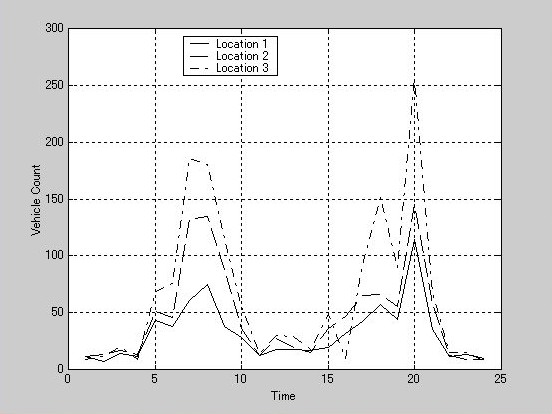
》 t = 1:n;
》 set(0,'defaultaxeslinestyleorder','-|--|-.')
》 set(0,'defaultaxescolororder',[0 0 0])
》 plot(t,count), legend('Location 1','Location 2','Location 3',0)
》 plot(t,count), legend('Location 1','Location 2','Location 3',0) xlable('Time'),ylabel('Vehicle Count'), grid on
??? cation 3',0) xlable
|
演算子、カンマ、またはセミコロンが見つかりません
》 plot(t,count), legend('Location 1','Location 2','Location 3',0) xlabel('Time'),ylabel('Vehicle Count'), grid on
??? cation 3',0) xlabel
|
演算子、カンマ、またはセミコロンが見つかりません
》 plot(t,count), legend('Location 1','Location 2','Location 3',0),xlabel('Time'),ylabel('Vehicle Count'), grid on
》 plot(t,count), legend('Location 1','Location 2','Location 3',0),xlabel('Time'),ylabel('Vehicle Count'), grid on
》 type count.dat
11 11 9
7 13 11
14 17 20
11 13 9
43 51 69
38 46 76
61 132 186
75 135 180
38 88 115
28 36 55
12 12 14
18 27 30
18 19 29
17 15 18
19 36 48
32 47 10
42 65 92
57 66 151
44 55 90
114 145 257
35 58 68
11 12 15
13 9 15
10 9 7
 基本數(shù)據(jù)分析
》 load count.dat
》 mx = max(count)
mx =
114 145 257
》 mu = mean(count)
mu =
32.0000 46.5417 65.5833
》 sigma = std(count)
sigma =
25.3703 41.4057 68.0281
》 [mx,indx] = min(count)
mx =
7 9 7
indx =
2 23 24
》 [n,p] =size(count)
n =
24
p =
3
》 e = ones(n,1)
e =
1
1
1
1
1
1
1
1
1
1
1
1
1
1
1
1
1
1
1
1
1
1
1
1
》 x = count - e*mu
x =
-21.0000 -35.5417 -56.5833
-25.0000 -33.5417 -54.5833
-18.0000 -29.5417 -45.5833
-21.0000 -33.5417 -56.5833
11.0000 4.4583 3.4167
6.0000 -0.5417 10.4167
29.0000 85.4583 120.4167
43.0000 88.4583 114.4167
6.0000 41.4583 49.4167
-4.0000 -10.5417 -10.5833
-20.0000 -34.5417 -51.5833
-14.0000 -19.5417 -35.5833
-14.0000 -27.5417 -36.5833
-15.0000 -31.5417 -47.5833
-13.0000 -10.5417 -17.5833
0 0.4583 -55.5833
10.0000 18.4583 26.4167
25.0000 19.4583 85.4167
12.0000 8.4583 24.4167
82.0000 98.4583 191.4167
3.0000 11.4583 2.4167
-21.0000 -34.5417 -50.5833
-19.0000 -37.5417 -50.5833
-22.0000 -37.5417 -58.5833
》 min(count(:))
ans =
7
協(xié)方差和對射變模
》 cov(count(:,1))
ans =
643.6522
》 corrcoef(count)
ans =
1.0000 0.9331 0.9599
0.9331 1.0000 0.9553
0.9599 0.9553 1.0000
》 A = [9 -2 3 0 1 5 4];
》 diff(A)
ans =
-11 5 -3 1 4 -1
數(shù)據(jù)預(yù)處理(Data Preprocessing)
》 mu = mean(count)
mu =
32.0000 46.5417 65.5833
》 sigma = std(count)
sigma =
25.3703 41.4057 68.0281
》 [n,p] = size(count)
n =
24
p =
3
》 outliers = abs(count - mu(ones(n,1),:)) > 3*sigma(ones(n,1),:);
》 nout = sum(outliers)
nout =
1 0 0
》 count(any(outliers'),:) = [];
回歸分析
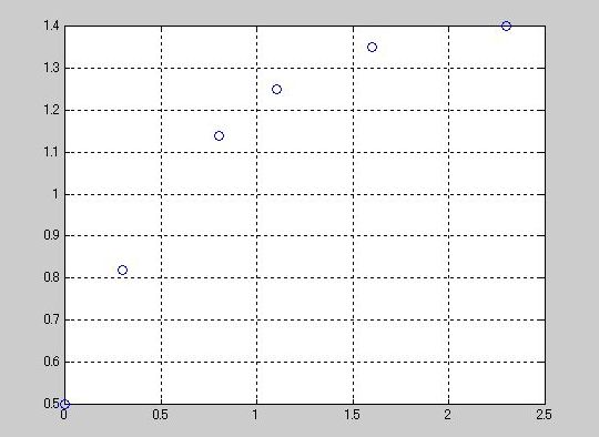
》 t = [0 .3 .8 1.1 1.6 2.3]';
》 y = [0.5 0.82 1.14 1.25 1.35 1.40]';
》 plot(t,y,'o'),grid on
基本數(shù)據(jù)分析
》 load count.dat
》 mx = max(count)
mx =
114 145 257
》 mu = mean(count)
mu =
32.0000 46.5417 65.5833
》 sigma = std(count)
sigma =
25.3703 41.4057 68.0281
》 [mx,indx] = min(count)
mx =
7 9 7
indx =
2 23 24
》 [n,p] =size(count)
n =
24
p =
3
》 e = ones(n,1)
e =
1
1
1
1
1
1
1
1
1
1
1
1
1
1
1
1
1
1
1
1
1
1
1
1
》 x = count - e*mu
x =
-21.0000 -35.5417 -56.5833
-25.0000 -33.5417 -54.5833
-18.0000 -29.5417 -45.5833
-21.0000 -33.5417 -56.5833
11.0000 4.4583 3.4167
6.0000 -0.5417 10.4167
29.0000 85.4583 120.4167
43.0000 88.4583 114.4167
6.0000 41.4583 49.4167
-4.0000 -10.5417 -10.5833
-20.0000 -34.5417 -51.5833
-14.0000 -19.5417 -35.5833
-14.0000 -27.5417 -36.5833
-15.0000 -31.5417 -47.5833
-13.0000 -10.5417 -17.5833
0 0.4583 -55.5833
10.0000 18.4583 26.4167
25.0000 19.4583 85.4167
12.0000 8.4583 24.4167
82.0000 98.4583 191.4167
3.0000 11.4583 2.4167
-21.0000 -34.5417 -50.5833
-19.0000 -37.5417 -50.5833
-22.0000 -37.5417 -58.5833
》 min(count(:))
ans =
7
協(xié)方差和對射變模
》 cov(count(:,1))
ans =
643.6522
》 corrcoef(count)
ans =
1.0000 0.9331 0.9599
0.9331 1.0000 0.9553
0.9599 0.9553 1.0000
》 A = [9 -2 3 0 1 5 4];
》 diff(A)
ans =
-11 5 -3 1 4 -1
數(shù)據(jù)預(yù)處理(Data Preprocessing)
》 mu = mean(count)
mu =
32.0000 46.5417 65.5833
》 sigma = std(count)
sigma =
25.3703 41.4057 68.0281
》 [n,p] = size(count)
n =
24
p =
3
》 outliers = abs(count - mu(ones(n,1),:)) > 3*sigma(ones(n,1),:);
》 nout = sum(outliers)
nout =
1 0 0
》 count(any(outliers'),:) = [];
回歸分析
》 t = [0 .3 .8 1.1 1.6 2.3]';
》 y = [0.5 0.82 1.14 1.25 1.35 1.40]';
》 plot(t,y,'o'),grid on
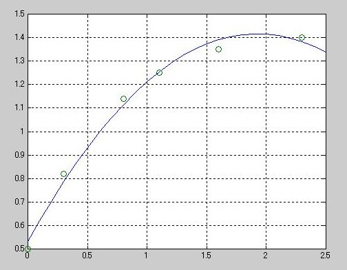
 多項(xiàng)式回歸分析
》 X = [ones(size(t)) t t.^2
]
X =
1.0000 0 0
1.0000 0.3000 0.0900
1.0000 0.8000 0.6400
1.0000 1.1000 1.2100
1.0000 1.6000 2.5600
1.0000 2.3000 5.2900
》 a = X\y
a =
0.5318
0.9191
-0.2387
》 T = (0:0.1:2.5)';
》 Y = [ones(size(T)) T T.^2]*a;
》 plot(T,Y,'-',t,y,'o'), grid on
多項(xiàng)式回歸分析
》 X = [ones(size(t)) t t.^2
]
X =
1.0000 0 0
1.0000 0.3000 0.0900
1.0000 0.8000 0.6400
1.0000 1.1000 1.2100
1.0000 1.6000 2.5600
1.0000 2.3000 5.2900
》 a = X\y
a =
0.5318
0.9191
-0.2387
》 T = (0:0.1:2.5)';
》 Y = [ones(size(T)) T T.^2]*a;
》 plot(T,Y,'-',t,y,'o'), grid on
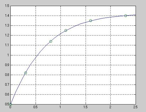
 線性回歸分析
》 X = [ones(size(t)) exp(- t) t.*exp(- t)];
》 a = X\y
a =
1.3974
-0.8988
0.4097
》 Y = [ones(size(T)) exp(- T) T.exp(- T)]*a;
??? Attempt to reference field of non-structure array 'T'.
》 T = (0:0.1:2.5)';
》 Y = [ones(size(T)) exp(- T) T.exp(- T)]*a;
??? Attempt to reference field of non-structure array 'T'.
》 T = (0:0.1:2.5)';
》 Y = [ones(size(T)) exp(- T) T.exp(- T)]*a;
??? Attempt to reference field of non-structure array 'T'.
》 Y = [ones(size(t)) exp(- t) T.exp(- t)]*a;
??? Attempt to reference field of non-structure array 'T'.
》 Y = [ones(size(t)) exp(- t) t.exp(- t)]*a;
??? Attempt to reference field of non-structure array 't'.
》 Y = [ones(size(T)) exp(- T) T.*exp(- T)]*a;
》 plot(T,Y,'-',t,y,'o'), grid on
線性回歸分析
》 X = [ones(size(t)) exp(- t) t.*exp(- t)];
》 a = X\y
a =
1.3974
-0.8988
0.4097
》 Y = [ones(size(T)) exp(- T) T.exp(- T)]*a;
??? Attempt to reference field of non-structure array 'T'.
》 T = (0:0.1:2.5)';
》 Y = [ones(size(T)) exp(- T) T.exp(- T)]*a;
??? Attempt to reference field of non-structure array 'T'.
》 T = (0:0.1:2.5)';
》 Y = [ones(size(T)) exp(- T) T.exp(- T)]*a;
??? Attempt to reference field of non-structure array 'T'.
》 Y = [ones(size(t)) exp(- t) T.exp(- t)]*a;
??? Attempt to reference field of non-structure array 'T'.
》 Y = [ones(size(t)) exp(- t) t.exp(- t)]*a;
??? Attempt to reference field of non-structure array 't'.
》 Y = [ones(size(T)) exp(- T) T.*exp(- T)]*a;
》 plot(T,Y,'-',t,y,'o'), grid on
 線性回歸分析
》 x1 = [.2 .5 .6 .8 1.0 1.1]';
》 x2 = [.1 .3 .4 .9 1.1 1.4]';
》 y = [.17 .26 .28 .23 .27 .24]';
》 X = [ones(size(xa) x1 x2];
??? = [ones(size(xa) x1
|
関數(shù)の參照が正しくありません。","、または ")" が足りません
》 X = [ones(size(x1)) x1 x2];
》 a = X\y
a =
0.1018
0.4844
-0.2847
》 Y = X*a;
》 MaxErr = max(abs(Y - y)
??? rr = max(abs(Y - y)
|
関數(shù)の參照が正しくありません。","、または ")" が足りません
》 MaxErr = max(abs(Y - y))
MaxErr =
0.0038
》 plot(T,Y,'-' t,y,'o'), grid on
??? plot(T,Y,'-' t
|
関數(shù)の參照が正しくありません。","、または ")" が足りません
》 T = (0:0.1:2.5)';
》 X
X =
1.0000 0.2000 0.1000
1.0000 0.5000 0.3000
1.0000 0.6000 0.4000
1.0000 0.8000 0.9000
1.0000 1.0000 1.1000
1.0000 1.1000 1.4000
》 plot(T,Y,'-',t,y,'o'), grid on
??? エラー: ==> plot
ベクトルは同じ長さである必要があります.
》 X = [ones(size(x1)) x1 x2];
》 a = X\y
a =
0.1018
0.4844
-0.2847
》 Y = X*a
Y =
0.1703
0.2586
0.2786
0.2332
0.2731
0.2362
》 plot(T,Y,'-',t,y,'o', grid on
??? -',t,y,'o', grid on
|
関數(shù)の參照が正しくありません。","、または ")" が足りません
》 plot(T,Y,'-',t,y,'o'), grid on
??? エラー: ==> plot
ベクトルは同じ長さである必要があります.
》 load census
》 p = polyfit(cdate,pop,4)
Warning: Matrix is close to singular or badly scaled.
Results may be inaccurate. RCOND = 5.429790e-020.
> In C:\MAT\toolbox\matlab\polyfun\polyfit.m at line 52
p =
1.0e+005 *
0.0000 -0.0000 0.0000 -0.0126 6.0020
》 sdate = (cdate -mean(cdate))./std(cdate)
sdate =
-1.6116
-1.4505
-1.2893
-1.1282
-0.9670
-0.8058
-0.6447
-0.4835
-0.3223
-0.1612
0
0.1612
0.3223
0.4835
0.6447
0.8058
0.9670
1.1282
1.2893
1.4505
1.6116
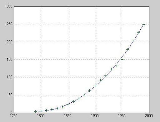
》 p = polyfit(sdate,pop,4)
p =
0.7047 0.9210 23.4706 73.8598 62.2285
》 pop4 = polyval(p,sdate);
》 plot(cdate,pop4,'-',cdate,pop,'+'), grid on
線性回歸分析
》 x1 = [.2 .5 .6 .8 1.0 1.1]';
》 x2 = [.1 .3 .4 .9 1.1 1.4]';
》 y = [.17 .26 .28 .23 .27 .24]';
》 X = [ones(size(xa) x1 x2];
??? = [ones(size(xa) x1
|
関數(shù)の參照が正しくありません。","、または ")" が足りません
》 X = [ones(size(x1)) x1 x2];
》 a = X\y
a =
0.1018
0.4844
-0.2847
》 Y = X*a;
》 MaxErr = max(abs(Y - y)
??? rr = max(abs(Y - y)
|
関數(shù)の參照が正しくありません。","、または ")" が足りません
》 MaxErr = max(abs(Y - y))
MaxErr =
0.0038
》 plot(T,Y,'-' t,y,'o'), grid on
??? plot(T,Y,'-' t
|
関數(shù)の參照が正しくありません。","、または ")" が足りません
》 T = (0:0.1:2.5)';
》 X
X =
1.0000 0.2000 0.1000
1.0000 0.5000 0.3000
1.0000 0.6000 0.4000
1.0000 0.8000 0.9000
1.0000 1.0000 1.1000
1.0000 1.1000 1.4000
》 plot(T,Y,'-',t,y,'o'), grid on
??? エラー: ==> plot
ベクトルは同じ長さである必要があります.
》 X = [ones(size(x1)) x1 x2];
》 a = X\y
a =
0.1018
0.4844
-0.2847
》 Y = X*a
Y =
0.1703
0.2586
0.2786
0.2332
0.2731
0.2362
》 plot(T,Y,'-',t,y,'o', grid on
??? -',t,y,'o', grid on
|
関數(shù)の參照が正しくありません。","、または ")" が足りません
》 plot(T,Y,'-',t,y,'o'), grid on
??? エラー: ==> plot
ベクトルは同じ長さである必要があります.
》 load census
》 p = polyfit(cdate,pop,4)
Warning: Matrix is close to singular or badly scaled.
Results may be inaccurate. RCOND = 5.429790e-020.
> In C:\MAT\toolbox\matlab\polyfun\polyfit.m at line 52
p =
1.0e+005 *
0.0000 -0.0000 0.0000 -0.0126 6.0020
》 sdate = (cdate -mean(cdate))./std(cdate)
sdate =
-1.6116
-1.4505
-1.2893
-1.1282
-0.9670
-0.8058
-0.6447
-0.4835
-0.3223
-0.1612
0
0.1612
0.3223
0.4835
0.6447
0.8058
0.9670
1.1282
1.2893
1.4505
1.6116
》 p = polyfit(sdate,pop,4)
p =
0.7047 0.9210 23.4706 73.8598 62.2285
》 pop4 = polyval(p,sdate);
》 plot(cdate,pop4,'-',cdate,pop,'+'), grid on
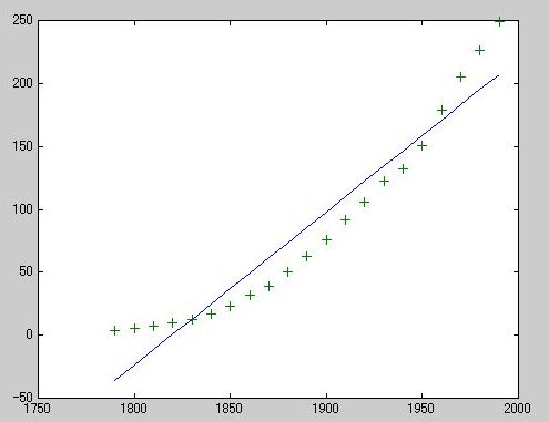
 》 p1 = polyfit(sdate,pop,1);
》 pop1 = polyval(p1,sdate);
》 plot(cdate,pop1,'-',cdate,pop,'+')
》 p1 = polyfit(sdate,pop,1);
》 pop1 = polyval(p1,sdate);
》 plot(cdate,pop1,'-',cdate,pop,'+')
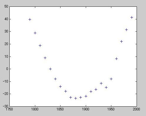
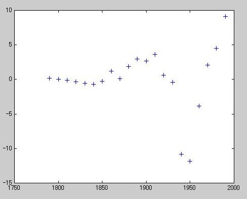
 》 res1 = pop - pop1;
》 figure, plot(cdate,res1,'+')
》 res1 = pop - pop1;
》 figure, plot(cdate,res1,'+')
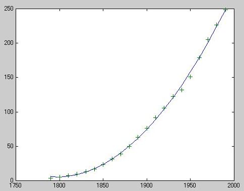
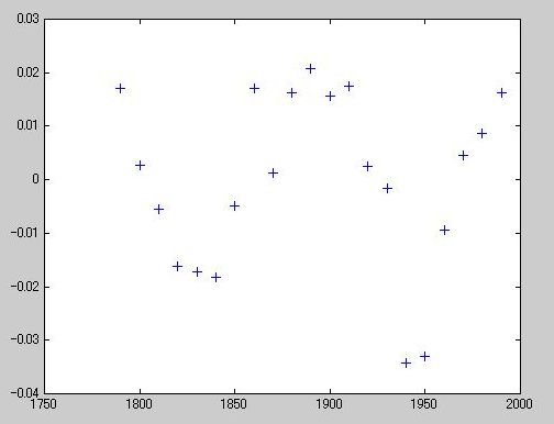
 》 p = polyfit(sdate,pop,2);
》 pop2 = polyval(p,sdate);
》 plot(cdate,pop2,'-',cdate,pop,'+')
》 p = polyfit(sdate,pop,2);
》 pop2 = polyval(p,sdate);
》 plot(cdate,pop2,'-',cdate,pop,'+')
 》 res2 = pop - pop2;
》 figure, plot(cdate,res2,'+')
》 res2 = pop - pop2;
》 figure, plot(cdate,res2,'+')
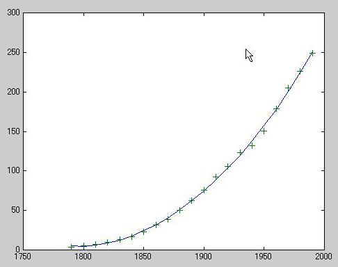
 》 p = polyfit(sdate,pop,4);
》 pop4 = polyval(p,sdate);
》 plot(cdate,pop4,'-',cdate,pop,'+')
》 p = polyfit(sdate,pop,4);
》 pop4 = polyval(p,sdate);
》 plot(cdate,pop4,'-',cdate,pop,'+')
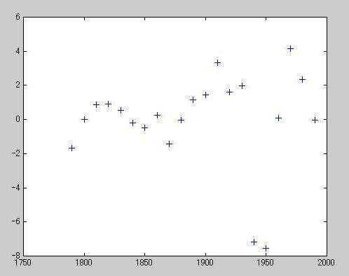
 》 res4 = pop - pop4;
》 figure,plot(cdate,res4,'+')
<img src="res32.jpg">
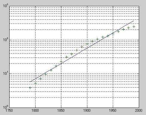
》 logp1 = polyfit(sdate,log10(pop),1);
》 logpred1 = 10.^polyval(logp1,sdate);
》 semilogy(cdate,logpred1,'-',cdate,pop,'+');
》 grid on
》 res4 = pop - pop4;
》 figure,plot(cdate,res4,'+')
<img src="res32.jpg">
》 logp1 = polyfit(sdate,log10(pop),1);
》 logpred1 = 10.^polyval(logp1,sdate);
》 semilogy(cdate,logpred1,'-',cdate,pop,'+');
》 grid on
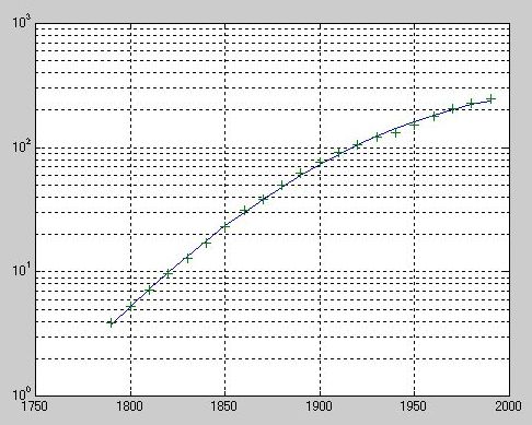
 》 logp2 = polyfit(sdate,log10(pop),2);
》 logpred2 = 10.^polyval(logp2,sdate);
》 semilogy(cdate,logpred2,'-',cdate,pop,'+'); grid on
》 logp2 = polyfit(sdate,log10(pop),2);
》 logpred2 = 10.^polyval(logp2,sdate);
》 semilogy(cdate,logpred2,'-',cdate,pop,'+'); grid on
 》 logres2 = log10(pop) - polyval(logp2,sdate);
》 plot(cdate,logres2,'+')
》 logres2 = log10(pop) - polyval(logp2,sdate);
》 plot(cdate,logres2,'+')
 》 r = pop - 10.^(polyval(logp2,sdate));
》 plot(cdate,r,'+')
》 r = pop - 10.^(polyval(logp2,sdate));
》 plot(cdate,r,'+')
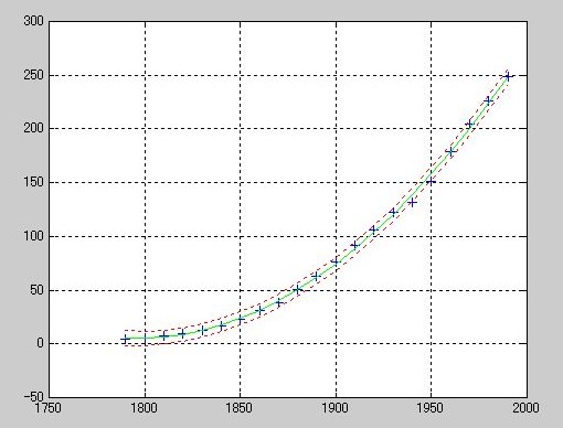
 plot(cdate,pop,'+',cdate,pop2,'g-',cdate,pop2+2*del2,'r:',cdate,pop2-2*del2,'r:'), grid on
 Fast Fourier Transform
》 x = [4 3 7 -9 1 0 0 0]';
》 y = fft(x)
y =
6.0000
11.4853 - 2.7574i
-2.0000 -12.0000i
-5.4853 +11.2426i
18.0000
-5.4853 -11.2426i
-2.0000 +12.0000i
11.4853 + 2.7574i
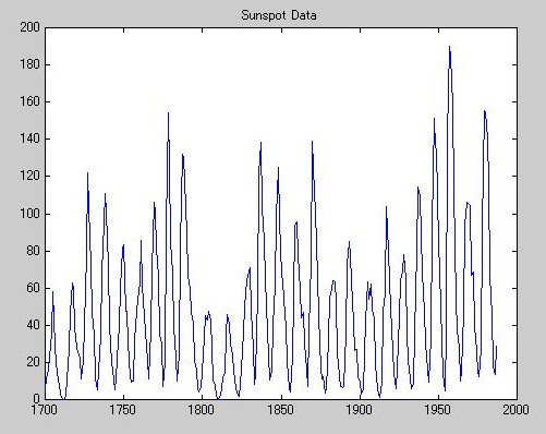
》 load sunspot.dat
》 year = sunspot(:,1);
》 wolfer = sunspot(:,2);
》 plot(year,wolfer)
》 title('Sunspot Data')
Fast Fourier Transform
》 x = [4 3 7 -9 1 0 0 0]';
》 y = fft(x)
y =
6.0000
11.4853 - 2.7574i
-2.0000 -12.0000i
-5.4853 +11.2426i
18.0000
-5.4853 -11.2426i
-2.0000 +12.0000i
11.4853 + 2.7574i
》 load sunspot.dat
》 year = sunspot(:,1);
》 wolfer = sunspot(:,2);
》 plot(year,wolfer)
》 title('Sunspot Data')
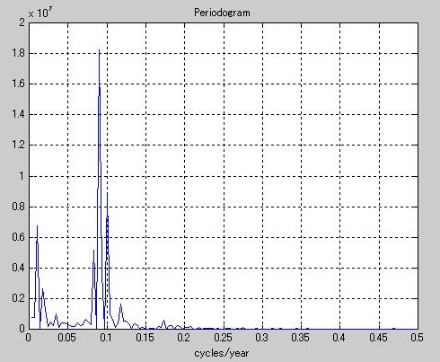
 》 Y = fft(wolfer);
》 N = length(Y);
》 Y(1) = [];
》 power = abs(Y(1:N/2)).^2;
》 nyquist = 1/2;
》 freq = (1:N/2)/(N/2)*nyquist;
》 plot(freq,power),grid on
》 xlabel('cycles/year')
》 title('Periodogram')
》 Y = fft(wolfer);
》 N = length(Y);
》 Y(1) = [];
》 power = abs(Y(1:N/2)).^2;
》 nyquist = 1/2;
》 freq = (1:N/2)/(N/2)*nyquist;
》 plot(freq,power),grid on
》 xlabel('cycles/year')
》 title('Periodogram')
 》 period = 1./freq;
》 plot(period,power), axis([0 40 0 2e7]), grid on
》 ylabel('Power')
》 xlabel('Period(Years/Cycle)')
》 period = 1./freq;
》 plot(period,power), axis([0 40 0 2e7]), grid on
》 ylabel('Power')
》 xlabel('Period(Years/Cycle)')
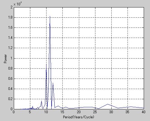 》 [mp index] = max(power);
》 period(index)
ans =
11.0769
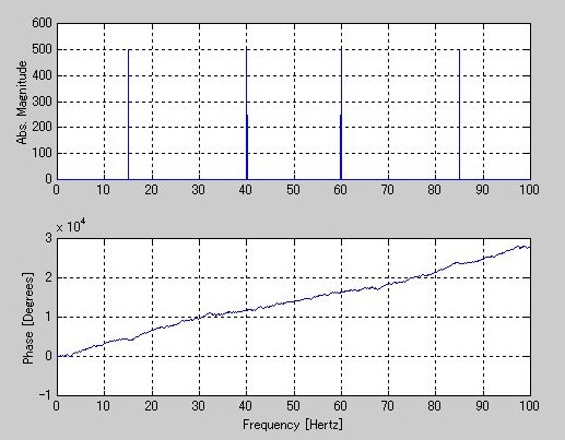
》 t = 0:1/100:10-1/100;
》 x = sin(2*pi*15*t) + sin(2*pi*40*t);
》 y = fft(x);
》 m = abs(y);
》 p = unwrap)angle(y));
??? p = unwrap)
|
演算子、カンマ、またはセミコロンが見つかりません
》 p = unwrap(angle(y));
》 f = (0:length(y)-1)'*100/length(y);
》 subplot(2,1,1), plot(f,m),
》 ylabel('Abs. Magnitude'), grid on
》 subplot(2,1,2), plot(f,p*180/pi)
》 ylabel('Phase [Degrees]'), grid on
》 xlabel('Frequency [Hertz]')
》 [mp index] = max(power);
》 period(index)
ans =
11.0769
》 t = 0:1/100:10-1/100;
》 x = sin(2*pi*15*t) + sin(2*pi*40*t);
》 y = fft(x);
》 m = abs(y);
》 p = unwrap)angle(y));
??? p = unwrap)
|
演算子、カンマ、またはセミコロンが見つかりません
》 p = unwrap(angle(y));
》 f = (0:length(y)-1)'*100/length(y);
》 subplot(2,1,1), plot(f,m),
》 ylabel('Abs. Magnitude'), grid on
》 subplot(2,1,2), plot(f,p*180/pi)
》 ylabel('Phase [Degrees]'), grid on
》 xlabel('Frequency [Hertz]')
返回
麟游县|
潜山县|
佳木斯市|
从化市|
三原县|
托克托县|
永善县|
商城县|
汽车|
宁明县|
文化|
南投市|
云浮市|
仪征市|
黑河市|
左权县|
海淀区|
阳城县|
盐源县|
濉溪县|
海晏县|
东台市|
乐昌市|
都兰县|
锡林郭勒盟|
图们市|
高陵县|
城市|
乐平市|
乌什县|
托克逊县|
五莲县|
独山县|
宁津县|
普宁市|
昌宁县|
荔浦县|
桦甸市|
加查县|
景泰县|
曲松县|